XGBoost Model Training

In this notebook, we will simulate the glacier surface mass balance for the Iceland region using a custom XGBoost model. The XGBoost model is designed with a custom objective function that generates monthly predictions based on aggregated observational data. We will create an instance of CustomXGBoostRegressor and train it using this custom loss function on the stake data from Iceland, which we have prepared in earlier notebooks. If you haven’t already, please review the data preprocessing and data preparation notebooks for more details.

The workflow includes several key steps:

1. Data Loading and Preparation: A Dataloader object is created to handle the loading of data and the creation of a training and testing split. This object also manages the generation of data splits for cross-validation.

2. Cross-Validation and Model Training: Using Scikit-learn’s cross-validation techniques, we explore different hyperparameters and train the model on the prepared data splits. This approach ensures a robust evaluation and helps in selecting suitable parameters.

3. Aggregated Predictions: After training, we will display the aggregated monthly predictions generated by the model to visualize and analyze the results.

4. Model Evaluation: Finally, the model’s performance is evaluated on the test set, providing insights into its predictive accuracy for glacier mass balance.

import pandas as pd
import massbalancemachine as mbm
import warnings
import seaborn as sns
import matplotlib.pyplot as plt
warnings.filterwarnings('ignore')
%load_ext autoreload
%autoreload 2

data = pd.read_csv('./example_data/iceland/files/iceland_monthly_dataset.csv')
print('Number of winter and annual samples:', len(data))
display(data)

cfg = mbm.Config()

Number of winter and annual samples: 442

	ELEVATION_DIFFERENCE	slope	MONTHS	POINT_ELEVATION	POINT_ID	YEAR	POINT_BALANCE	N_MONTHS	POINT_LAT	RGIId	...	POINT_LON	aspect	ID	t2m	tp	slhf	sshf	ssrd	fal	str
0	116.476388	0.041035	oct	1450.4	hn14aa	1995	2.07	8	64.885013	RGI60-06.00228	...	-18.773871	5.810070	0	267.885682	0.005071	-32688.346894	1.908546e+05	3.434260e+06	0.850005	-1.029337e+06
1	116.476388	0.041035	nov	1450.4	hn14aa	1995	2.07	8	64.885013	RGI60-06.00228	...	-18.773871	5.810070	0	266.376346	0.006053	301104.083653	8.280538e+05	8.424995e+05	0.849992	-1.431540e+06
2	116.476388	0.041035	dec	1450.4	hn14aa	1995	2.07	8	64.885013	RGI60-06.00228	...	-18.773871	5.810070	0	263.049011	0.005854	248241.745197	9.954409e+05	1.322171e+05	0.849992	-2.002829e+06
3	116.476388	0.041035	jan	1450.4	hn14aa	1995	2.07	8	64.885013	RGI60-06.00228	...	-18.773871	5.810070	0	261.692810	0.004156	348585.225978	1.243700e+06	4.884578e+05	0.849992	-1.792889e+06
4	116.476388	0.041035	feb	1450.4	hn14aa	1995	2.07	8	64.885013	RGI60-06.00228	...	-18.773871	5.810070	0	261.140088	0.002287	274514.643950	1.004845e+06	2.580602e+06	0.850005	-1.861757e+06
...	...	...	...	...	...	...	...	...	...	...	...	...	...	...	...	...	...	...	...	...	...
437	-246.593874	0.067458	may	821.0	blt8	2018	-2.63	12	64.662707	RGI60-06.00232	...	-18.954942	3.476423	54	271.553741	0.006217	-264554.591916	3.063329e+05	2.073085e+07	0.826504	-2.648321e+06
438	-246.593874	0.067458	jun	821.0	blt8	2018	-2.63	12	64.662707	RGI60-06.00232	...	-18.954942	3.476423	54	276.144439	0.003192	10994.304045	6.234279e+05	1.787212e+07	0.768536	-9.177811e+05
439	-246.593874	0.067458	jul	821.0	blt8	2018	-2.63	12	64.662707	RGI60-06.00232	...	-18.954942	3.476423	54	277.553280	0.003422	-589325.605420	7.537638e+04	1.425122e+07	0.676787	-7.246837e+05
440	-246.593874	0.067458	aug	821.0	blt8	2018	-2.63	12	64.662707	RGI60-06.00232	...	-18.954942	3.476423	54	276.193729	0.002495	-807105.778219	-1.563324e+05	1.332676e+07	0.677706	-1.884936e+06
441	-246.593874	0.067458	sep	821.0	blt8	2018	-2.63	12	64.662707	RGI60-06.00232	...	-18.954942	3.476423	54	273.151130	0.003491	-432479.565272	1.434597e+05	9.078256e+06	0.717923	-2.152404e+06

442 rows × 21 columns

1. Create the train and test datasets and the data splits for Cross Validation

First, we create a DataLoader object, which generates both training and testing datasets, as well as the data splits required for cross-validation (CV). To conserve memory, the set_train_test_split method returns iterators containing indices for the training and testing datasets. These indices are then used to retrieve the corresponding data for training and testing. Next, the get_cv_split method provides a list indicating the number of folds needed for cross-validation.

# Create a new DataLoader object with the monthly stake data measurements.
dataloader = mbm.dataloader.DataLoader(cfg, data=data)
# Create a training and testing iterators. The parameters are optional. The default value of test_size is 0.3.
train_itr, test_itr = dataloader.set_train_test_split(test_size=0.3)

# Get all indices of the training and testing dataset at once from the iterators. Once called, the iterators are empty.
train_indices, test_indices = list(train_itr), list(test_itr)

# Get the features and targets of the training data for the indices as defined above, that will be used during the cross validation.
df_X_train = data.iloc[train_indices]
y_train = df_X_train['POINT_BALANCE'].values

# Get test set
df_X_test = data.iloc[test_indices]
y_test = df_X_test['POINT_BALANCE'].values

# Create the cross validation splits based on the training dataset. The default value for the number of splits is 5.
splits = dataloader.get_cv_split(n_splits=5)

# Print size of train and test
print(f"Size of training set: {len(train_indices)}")
print(f"Size of test set: {len(test_indices)}")

feature_columns = df_X_train.columns.difference(cfg.metaData)
feature_columns = feature_columns.drop(cfg.notMetaDataNotFeatures)
feature_columns = list(feature_columns)
cfg.setFeatures(feature_columns)

Size of training set: 299
Size of test set: 143

2. Create a CustomXGBoostRegressor model

Next, we define the parameter ranges for each XGBoost parameter. In the subsequent step, we use cross-validation to explore these parameter ranges and select the combination that yields the lowest loss. Additionally, we create a CustomXGBoostRegressor object.

# For each of the XGBoost parameter, define the grid range
parameters = {
    'max_depth': [
        3,
        4,
        5,
    ],
    'learning_rate': [0.01, 0.1],
    'n_estimators': [200, 300],
    'gamma': [0, 1]
}

# Create a CustomXGBoostRegressor instance
params_init = {"device": "cpu"}
custom_xgboost = mbm.models.CustomXGBoostRegressor(cfg, **params_init)

3. Training

In the following cell, we begin training our model using either GridSearchCV or RandomizedSearchCV:

• GridSearchCV performs an exhaustive search across all possible parameter combinations to find the best set for optimal performance using cross-validation. While this method is thorough, it is often time-consuming and computationally expensive.

• RandomizedSearchCV, on the other hand, samples a fixed number of parameter combinations from the distribution, making it more efficient in terms of time and computational resources, especially with larger hyperparameter spaces. However, this approach may miss some of the best parameter combinations that aren’t selected in the random sampling.

You can choose either of the two training methods. Both methods will use all CPU cores by default. If you want to adjust the number of cores used, you can change the num_jobs parameter in the cfg instance.

# GridSearch
# custom_xgboost.gridsearch(parameters=parameters, splits=splits, features=df_X_train, targets=y_train)

# RandomisedSearch, with n_iter the number of parameter settings that are sampled. Trade-off between goodness of the solution
# versus runtime.
custom_xgboost.randomsearch(
    parameters=parameters,
    n_iter=5,
    splits=splits,
    features=df_X_train,
    targets=y_train,
)
best_params = custom_xgboost.param_search.best_params_
best_estimator = custom_xgboost.param_search.best_estimator_
print("Best parameters:\n", best_params)
print("Best score:\n", custom_xgboost.param_search.best_score_)

Fitting 5 folds for each of 5 candidates, totalling 25 fits
Best parameters:
 {'n_estimators': 300, 'max_depth': 3, 'learning_rate': 0.01, 'gamma': 1}
Best score:
 -0.6256725645604282

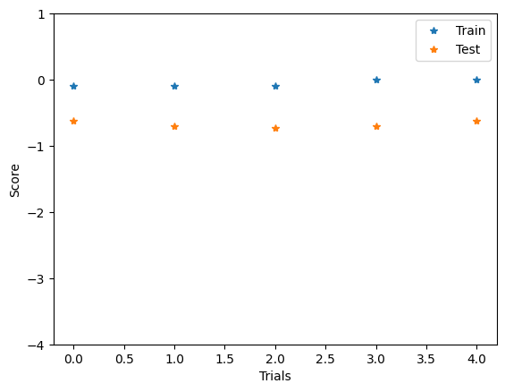
We can visualize the score associated to each of the candidates on both the training and testing sets. Because the optimization can diverge depending on the values of the hyper-parameters (such as the learning rate), we can obtain very large values. We filter out these values by limiting the y axis to realistic score values.

plt.plot(custom_xgboost.param_search.cv_results_['mean_train_score'], linestyle='', marker='*', label="Train")
plt.plot(custom_xgboost.param_search.cv_results_['mean_test_score'], linestyle='', marker='*', label="Test")
plt.legend()
plt.xlabel("Trials")
plt.ylabel("Score")
plt.ylim((-4, 1))
plt.show()

3.1 Save the trained model

# custom_xgboost.save_model('model.pkl')

# mbm.models.CustomXGBoostRegressor.load_model('model.pkl')

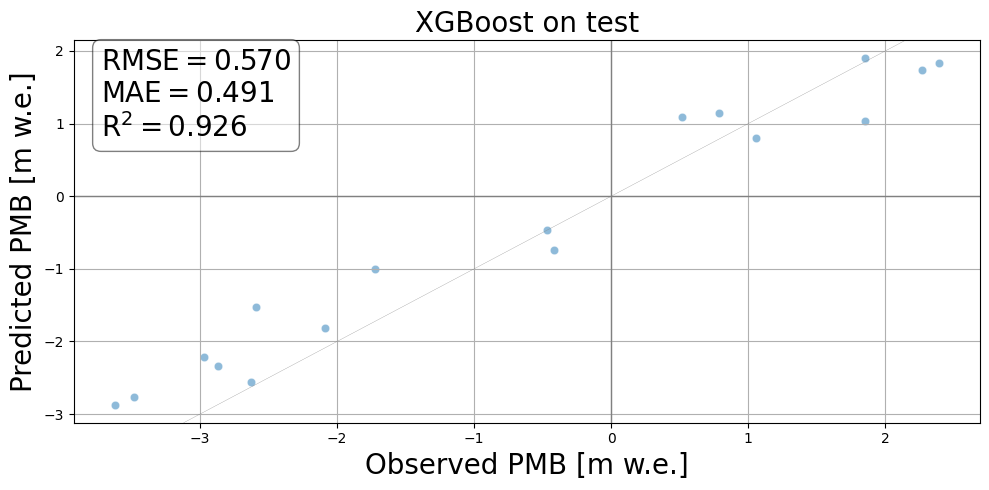
3.2 Show the predictions

# Set to CPU for predictions:
xgb = best_estimator.set_params(device='cpu')

# Make predictions on test
features_test, metadata_test = mbm.data_processing.utils.create_features_metadata(cfg, df_X_test)
y_pred = xgb.predict(features_test)

# Make predictions aggr to meas ID:
y_pred_agg = xgb.aggrPredict(metadata_test, features_test)

# Calculate scores
score = xgb.score(df_X_test, y_test)  # negative
mse, rmse, mae, pearson, r2, bias = xgb.evalMetrics(metadata_test, y_pred, y_test)

# Aggregate predictions to annual or winter:
df_pred = df_X_test.copy()
df_pred['target'] = y_test
grouped_ids = df_pred.groupby('ID').agg({'target': 'mean', 'RGIId': 'first'})
grouped_ids['pred'] = y_pred_agg

scores = {'rmse': rmse, 'mae': mae, 'R2': r2}
fig = mbm.plots.predVSTruth(
    grouped_ids,
    scores=scores,
    marker="o",
    title='XGBoost on test',
    alpha=0.5,
)

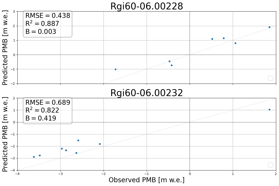
3.3 Show the predictions per glacier

scores = {}
for i, test_gl in enumerate(grouped_ids["RGIId"].unique()):
    df_gl = grouped_ids[grouped_ids["RGIId"] == test_gl]
    glacier_scores = mbm.metrics.scores(df_gl["target"], df_gl["pred"])
    scores[test_gl] = {
        "rmse": glacier_scores["rmse"],
        "R2": glacier_scores["r2"],
        "B": glacier_scores["bias"],
    }

fig, axs = plt.subplots(2, 1, figsize=(12, 8), sharex=True)
mbm.plots.predVSTruthPerGlacier(
    grouped_ids,
    axs=axs,
    scores=scores,
)