Data Exploration
In this notebook, we will introduce several plotting methods to help you analyze the stake measurement dataset you created during data preparation. The MassBalanceMachine library currently provides two types of plotting methods:
First, it allows you to plot a point surface mass balance timeseries for all stakes across all measured years. This includes the region-wise mean and standard deviation of the point surface mass balance. Second, it enables you to plot a region-wide cumulative annual surface mass balance for the available stakes in the dataset.
We plan to add more data visualization options in future releases of MassBalanceMachine. If you have suggestions for new visualizations that would benefit other users or are specific to a certain region, please feel free to create new GitHub issues or submit pull requests.
Note: It is assumed that the column names in the dataset resemble those in the WGMS files. If this isn’t the case, please refer to either the data preprocessing notebook or the data preparation notebook for guidance.
[1]:
import pandas as pd
import massbalancemachine as mbm
[2]:
data = pd.read_csv('./example_data/iceland/files/iceland_monthly_dataset.csv')
display(data)
| YEAR | POINT_LON | POINT_LAT | POINT_BALANCE | ALTITUDE_CLIMATE | ELEVATION_DIFFERENCE | POINT_ELEVATION | RGIId | POINT_ID | ID | ... | MONTHS | aspect | slope | t2m | tp | slhf | sshf | ssrd | fal | str | |
|---|---|---|---|---|---|---|---|---|---|---|---|---|---|---|---|---|---|---|---|---|---|
| 0 | 1995 | -18.773871 | 64.885013 | 2.07 | 1333.923612 | 116.476388 | 1450.4 | RGI60-06.00228 | hn14aa | 0 | ... | oct | 1.606406 | 0.056246 | 267.885682 | 0.005071 | -32688.346894 | 1.908546e+05 | 3.434260e+06 | 0.850005 | -1.029337e+06 |
| 1 | 1995 | -18.773871 | 64.885013 | 2.07 | 1333.923612 | 116.476388 | 1450.4 | RGI60-06.00228 | hn14aa | 0 | ... | nov | 1.606406 | 0.056246 | 266.376346 | 0.006053 | 301104.083653 | 8.280538e+05 | 8.424995e+05 | 0.849992 | -1.431540e+06 |
| 2 | 1995 | -18.773871 | 64.885013 | 2.07 | 1333.923612 | 116.476388 | 1450.4 | RGI60-06.00228 | hn14aa | 0 | ... | dec | 1.606406 | 0.056246 | 263.049011 | 0.005854 | 248241.745197 | 9.954409e+05 | 1.322171e+05 | 0.849992 | -2.002829e+06 |
| 3 | 1995 | -18.773871 | 64.885013 | 2.07 | 1333.923612 | 116.476388 | 1450.4 | RGI60-06.00228 | hn14aa | 0 | ... | jan | 1.606406 | 0.056246 | 261.692810 | 0.004156 | 348585.225978 | 1.243700e+06 | 4.884578e+05 | 0.849992 | -1.792889e+06 |
| 4 | 1995 | -18.773871 | 64.885013 | 2.07 | 1333.923612 | 116.476388 | 1450.4 | RGI60-06.00228 | hn14aa | 0 | ... | feb | 1.606406 | 0.056246 | 261.140088 | 0.002287 | 274514.643950 | 1.004845e+06 | 2.580602e+06 | 0.850005 | -1.861757e+06 |
| ... | ... | ... | ... | ... | ... | ... | ... | ... | ... | ... | ... | ... | ... | ... | ... | ... | ... | ... | ... | ... | ... |
| 440 | 2018 | -18.954942 | 64.662707 | -2.63 | 1067.593874 | -246.593874 | 821.0 | RGI60-06.00232 | blt8 | 54 | ... | jun | 2.889730 | 0.018996 | 276.144439 | 0.003192 | 10994.304045 | 6.234279e+05 | 1.787212e+07 | 0.768536 | -9.177811e+05 |
| 441 | 2018 | -18.954942 | 64.662707 | -2.63 | 1067.593874 | -246.593874 | 821.0 | RGI60-06.00232 | blt8 | 54 | ... | jul | 2.889730 | 0.018996 | 277.553280 | 0.003422 | -589325.605420 | 7.537638e+04 | 1.425122e+07 | 0.676787 | -7.246837e+05 |
| 442 | 2018 | -18.954942 | 64.662707 | -2.63 | 1067.593874 | -246.593874 | 821.0 | RGI60-06.00232 | blt8 | 54 | ... | aug | 2.889730 | 0.018996 | 276.193729 | 0.002495 | -807105.778219 | -1.563324e+05 | 1.332676e+07 | 0.677706 | -1.884936e+06 |
| 443 | 2018 | -18.954942 | 64.662707 | -2.63 | 1067.593874 | -246.593874 | 821.0 | RGI60-06.00232 | blt8 | 54 | ... | sep | 2.889730 | 0.018996 | 273.151130 | 0.003491 | -432479.565272 | 1.434597e+05 | 9.078256e+06 | 0.717923 | -2.152404e+06 |
| 444 | 2018 | -18.954942 | 64.662707 | -2.63 | 1067.593874 | -246.593874 | 821.0 | RGI60-06.00232 | blt8 | 54 | ... | oct_ | 2.889730 | 0.018996 | 269.734786 | 0.006109 | 108805.457235 | 5.504547e+05 | 3.653722e+06 | 0.834920 | -1.553769e+06 |
445 rows × 21 columns
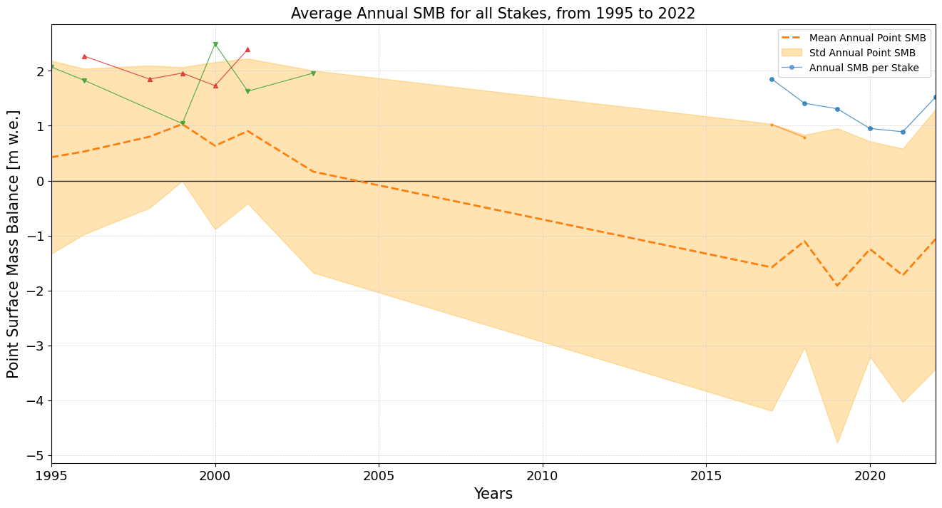
1. Plot the Point Surface Mass Balance for all Available Stakes
In this section, we will generate a plot for the point surface mass balance timeseries for all available stakes across all measured years. The plot will also include the region-wise mean and standard deviation of the point surface mass balance, providing a comprehensive view of the data’s temporal and regional trends.
[3]:
mbm.data_processing.utils.plot_stake_timeseries(data, ['svg', './example_data/iceland/plots/'])
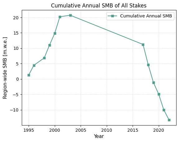
2. Plot the Cumulative Region-Wide Surface Mass Balance
In this section, we will create a plot to visualize the cumulative annual surface mass balance for a single region. This plot will aggregate the data from all available stakes within the region, offering insights into the overall mass balance trends over time.
[4]:
mbm.data_processing.utils.plot_cumulative_smb(data, ['svg', './example_data/iceland/plots/'])